18.1 Sulfur in crop nutrition

Plants take up sulfur (S) from the soil solution via their roots. Sulfur is taken up primarily in the form of sulfate (SO₄²⁻), although it is possible for plants to absorb SO₂ gas through their leaves. This secondary for of S uptake occurs at a much lower rate and contributes far less to the total S taken up by the plant compared what is taken up by the roots. Once inside the plant the sulfate will either be reduced to sulfide and attached to a carbon skeleton (similar to the process of ammonium uptake and movement throughout the plant) or remain as sulfate and be transported upwards through the plant and stored in a plant cell vacuole. In order for the plant cells and cell organelles to use the S, they need to first reduce it to sulfide. This reduction does not happen upon uptake; instead, after uptake the sulfate is only reduced to fulfill plant demand, whereupon it is immediately used by the plant cells and organelles.

Sulfur transporters facilitate the movement of the sulfate out of the aqueous transpiration stream flowing through the xylem cells and into the plant cells that surround them. Whereupon, additional S transporters can then translocate it into specific organelles. Sulfur is essential for plant growth and metabolism. Without it, plants would not be able to synthesize the S-containing amino acids: cysteine, cystine and methionine; each of which are necessary for the formation and function of enzymes and proteins (especially structural proteins) inside the plant. Sulfur also plays a critical role in the formation of sulfo-lipids, and can serve as a cofactor in several enzymatic processes. Sulfur is considered an immobile nutrient once it enters the plant. After the sulfate is taken up by the roots and transported upward through the xylem in the transpiration stream and into the plant cells, it is immobilized upon its incorporation into amino acids and other S-containing compounds. However, under severe nitrogen deficiency, plants may begin to break down nitrogen compounds that may contain S (such as proteins) to satisfy its N requirement. This deconstruction releases sulfate and other S-containing compounds, which can then move together with the newly mobilized nitrogen throughout the phloem. An excellent review of S’s role in cysteine metabolism is provided by Hoefgen and Hesse (2008).

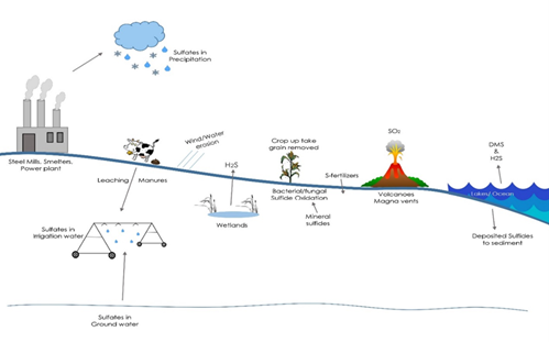
Sulfur is one of the fourteen essential mineral nutrients that all crops need. Figure 18.1 illustrates the S cycle on a large spatial scale. The S that plants use comes from two primary sources: anthropogenic and natural S. Anthropogenic S sources can be substantial, and include all emissions of sulfur dioxide (SO₂), hydrogen sulfide (H₂S), and a lesser amount of carbonyl sulfide (COS). Natural sources of atmospheric S include volcanic emissions, including magma vents which emit H₂S, oceans and other surface waters which emit H₂S and COS, atmospheric chemical reactions that transform H₂ S and COS into sulfuric acid (H₂SO₄), and manure emissions. Soil sources of S include degradation of S-bearing minerals, mineralization of plant residues and animal decay, formation and dissolution of sulfate salts, and the movement of sulfate-containing groundwater to the soil surface through irrigation or water table fluctuation. In S-deficient environments, S-inputs such as fertilizers and manures can improve crop production.

Figure 18.1 Sulfur cycle in air, water and soil (Franzen).

18.2 Natural sulfur sources

18.2.1 Volcanic activity

There were about 380 recorded active volcanoes within the past century, and typically in any given year there is at least 50 active volcanoes (Textor et al., 2003). Most of the volcanic activity across the globe is clustered into several active seismic regions, with the majority of the volcanic activity in North America is concentrated in the western mountains. The closest source of volcanic activity to the north central region of the United States is the Yellowstone Caldera, which last erupted about 600,000 years ago creating Yellowstone National Park as we know it. To this day in Yellowstone, there are many magma-heated areas of the National Park that still have significant amounts of magma close enough to the surface to where large amounts of S gasses are continually emitted, and can be easily smelled by tourists. All of the magma in the Yellowstone basin region is basaltic in nature, and as such the gasses it gives off, whether during eruption or through magma vents, contain large amounts of S compounds. Ninety percent of all volcanoes that erupt annually have basaltic magma, and 90 percent of these are located on the ocean floor (Halmer et al., 2002). Felsic magma, in contrast, is highly differentiated and contains a higher concentration of dissolved gases, including S compounds. This magma is both highly viscous and explosive. Andesitic magma is similar to felsic magma in both its viscosity and explosive nature, but is specifically found at convergent plate boundaries. The explosiveness of a volcanic eruptions can release large quantities of both magma and gas in a very short time period. These powerful eruptions can propel gasses 25 miles+ upwards into the stratosphere at incredible velocities. Volcanoes can also continuously emit gases through vents in between the large eruption events. The estimated annual S gas release by volcanic activity is shown in Table 18.1.

18.2.1.1 Table 18.1 Sulfur gases emitted annually by volcanic activity over the past 100 years (From Textor et al., 2003).

Species	SO₂	H₂S	COS	CS₂
Percent by volume	1–25	1–10	10⁻⁴–10⁻²	10⁻⁴–10⁻²
1,000 tons per year	1,650–55,000	1,100–3,100	7–110	8–105

When you average the total annual S-emission volume, the mean value masks the extreme volumes of S released into the upper atmosphere during the individual, catastrophic —but brief— eruptions. The Mt. St. Helens eruption in 1980 alone resulted in over 1.1 million tons of SO2 emissions. The Pinatubo eruption in the Philippines in 1991 released even more SO2 exceeding over 18.7 million tons. The largest recorded SO₂ emission during the past 250 years was from the Tambora eruption in Indonesia in 1815, resulting in an estimated 143 million tons of SO₂ being emitted. Once in the atmosphere the sulfur dioxide is transformed to sulfuric acid within about 35 days (Bluth et al., 1992). Sulfur from volcanoes makes up an estimated (Graf et al., 1997) 14 per cent of the total global gaseous S-emissions that occur annually. Total volcanic activity has increased during the past 30 years; however, this trend has been attributed more to improved monitoring and detection than any actual increase in overall activity (Halmer et al., 2002).
The transformation of sulfur dioxide to sulfuric acid in the atmosphere is described by the following formula (Manahan, S.E. 2013): \[ 2SO_2 + O_2 + 2H_2O \rightarrow 2H_2SO_4 \] The source of the water in the reaction is the ambient water vapor, which is greatly increased by the massive amounts of water vapor that is released during volcanic eruptions (Joshi & Jones, 2009).

18.2.2 Gas emission from surface waters

Oceans also emit large amounts of S gases that contribute to the overall background S concentrations of the atmosphere. One estimate of the total amount of S emitted from oceans as gas annually, is about 2 million tons. In addition, particulate S emitted from sea-spray is estimated to be about 10 million tons per year (Andreae, 1990). Sulfur taken up by marine algae is released as dimethyl sulfonium propionate, which is then further transformed to dimethyl sulfide (DMS). A portion of this DMS will diffuse into the atmosphere, where it is then oxidized back into sulfate (Andreae, 1990). The oxidation of DMS is a very complex process and proceeds as purely physical chemical reactions. An excellent review of the steps in the oxidation of DMS, the associated kinetics, and several accompanying flow charts can be found in Barnes et al. (2006). Coastal wetlands across the globe, such as the mangrove swamps in Florida, also emit S at a rate of about 2.1 million tons per year. Isolated regions of larger S gas emissions in the ocean can occur due when anoxic (no oxygen) zones are formed, usually near a continental shelf (Weeks et al., 2004). These coastal S emitting zones were once thought to only form as a result of small intermittent eruptions of H₂S in these waters; however, remote imagery now has revealed that these eruptions occur over vast tracts, sometimes reaching more than 5 million acres in total area (Figure 18.2).

Figure 18.2 Hydrogen sulfide eruptions from continental shelf sulfate reduction off the coast of Namibia, Africa; green areas in water to the left of the brown coastal area. (NASA Earth Observatory, 2010).

Although far greater global S gases are emitted by oceans compared to fresh water sources, fresh water lakes and wetlands found in North America can also emit S gases. In fresh water wetlands —which are common to many areas of North Dakota, South Dakota, Minnesota, Wisconsin, Michigan and the Prairie Provinces of Canada— the rate of gasses emitted that contain sulfur compounds (mostly H2S and DMS) can vary widely depending on the total size of the body of water. On average, however, the rate is calculated to be about 2 pounds of S per acre of water per year. In contrast, saltmarshes and other ocean associated wetlands, such as the mangrove swamps of Florida, can emit well over 20 pounds S per acre of water per year (Giblin & Wieder, 1992).

18.2.3 Sulfur-bearing minerals

The origin of most S in soils comes from the rocky parent material. The type of rocks that contain S in the USA includes igneous, magmatic, and sedimentary type rocks. Igneous rock can contain differing amounts of S in several different forms; with sulfides being the most abundant. These sulfides occur mainly as pyrites, iron pyrite (FeS₂) and pyrrhotite (Fe₁₋ₓS), but can also occur in smaller quantities in other S- bearing minerals (Parat et al., 2011). Small amounts of sulfates can also be present in some magmatic rocks, but these are also largely dominated by sulfides; however, significant weathering can change this ratio. Sedimentary rocks are themselves the products of previous ancient weathering/reconstitution events, and as such can contain a range of different S compounds, synthesized from various chemical sulfate reactions and S reductions (Rickard, 2012). Most of the mineral portions of our soils are a combination of igneous and sedimentary rocks and their weathered products.

Sulfates are present in the soils across the Great Plains region in the forms of sulfate salts including calcium, magnesium and sodium salts. Despite the large gypsum (CaSO₄ • 2 2H₂O) beds mined in many areas across the region, which are the direct products of ocean shoreline chemistry millions of years ago (Murray, 1964), as a whole the sulfate salts in the soils of North Dakota, northwest Minnesota and South Dakota are primarily the products of more recent evaporation chemistry events (Skarie et al., 1987). Sulfate salts dominate the ground water chemistry in North Dakota. The exceptions to this are areas near Grand Forks, where artesian water from ancient shale seabed strata has resulted in high quantities of chloride salts and is responsible for the “salt-flat” like appearance of land directly west of the city.

The sulfate dominated soluble salts found in the soil of North Dakota impacts most crop, pasture and rangeland production across the state. Sulfate salts also dominate most saline areas of Kansas (Whittemore, 2000), Nebraska (Joeckel and Clement, 2005), and South Dakota (Kennedy, 1994). Across North Dakota, summer evaporation typically exceeds precipitation most years. As a result, the groundwater moves upwards via capillary action into the surface soils, bringing its dissolved salts along with it. One positive side effect of this process is that crops grown in the areas that are typically negatively affected by sulfate salts rarely have any S deficiencies. However, the negative side to this process is that soluble salts can limit yield, and can eventually lead to the complete sterilization of the land if not managed well (Franzen, 2003). Surface evaporation of the groundwater is the main cause of elevated sulfate levels at the soil surface, although soil freezing can also cause the precipitation of sulfate salts (Arndt and Richardson, 1989). Salinity problems can be, by and large, an ephemeral issue (i.e. temporary, or of a short duration) (Franzen, 2003). For instance, during periods of high rainfall, followed by dry weather, the water-table will rise and salts are then pulled to the surface by capillary action, increasing the concentration of salts and sulfates in the crop rooting zone. Contrastingly, during periods of high rainfall in soils with either temporal or permanent deep water- tables, the sulfates are leached out of the rooting zone.

18.3 Anthropogenic sources of S gas emission

The main sources of anthropogenic S in the atmosphere, and the S cycle as a whole, are the emissions from oil, gas and coal-fired power plants, steel mills and smelters, grassland burning, crop residue burning, land clearing of forests by burning, and irrigation with sulfate-containing water. Coal has been used in by humans for over 2,000 years. Theophrastus (300 BC) writes of coal being mined in ancient Greece to be used by Greek metal workers. In China, coal was called “black stone” and appeared in their written records around 2,000 years ago during the Han dynasty. It was then described by Marco Polo during his historic journey to China about 1300 AD (Yinke, 2011). It is, however, very unlikely that the coal burning activities of these ancient societies could have significantly increased the overall global atmospheric sulfur levels. It was not until about 200 years ago, soon after the onset of the Industrial Revolution, that initially coal, then oil, then gas, were burned at a much larger scale (Fernihough and O’Rourke, 2014; Mokyr, 1998).
The Industrial Revolution is characterized by the mass-replacement of human and animal power with water and chemical power from timber, charcoal and coal. However, with limited sources of water power and trees the exponential increase in demand from the ever-burgeoning industry required additional sources of power that could be brought to the factories. Initially starting in Europe and expanding across the globe, coal and then oil products, filled that role. From early in the Industrial Revolution until today, the burning of fossil fuels has become the greatest single contributor to global atmospheric S concentration. For example, Chicago was an area that between 1921-1923 was littered with multiple steel mills, smelters, coal-powered power plants, coal-heated households, and many other industries that were powered by the burning of coal. Sulfur levels in the rainwater in Chicago during that time period measured 209 pounds S per acre. In comparison, the rainwater collected in 1921 in and around Ames, IA (an area at the time that had seen little industrialization other than coal-heated homes) measured 15 pounds S per acre (Eriksson, 1952).

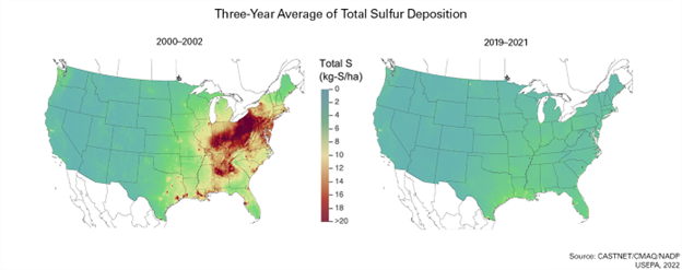
The US Clean Air Act of 1990 gave the US-EPA authority to reduce the toxic gas emissions into the atmosphere by regulating all of the gas emitting industries (U.S. Environmental Protection Agency, 2015). Using the 1980 SO₂ emission levels as a benchmark, Title IV of the Clean Air Act set a goal of reducing the total SO₂ emissions from coal-burning electric utilities by 10 million tons (Phase 1, 1995). It then further mandated the reductions of additional industries powered by coal, oil and gas (Phase II, 2000). The progressive effect of the successful implementation of the Clean Air Act is shown in the S deposition maps from 2000-2002 and 2019-2021 (Figure 18.3). The current total number of coal-fired industries in the North Central US states in the year 2015 are listed in Table 18.2. These values reflect the total emissions from all of the regions power plants, and other coal/oil/gas powered industries; such as the American Crystal Sugar sugarbeet processing plants in North Dakota. The site density of coal-fired industry units increases as you move from west to east across the region.

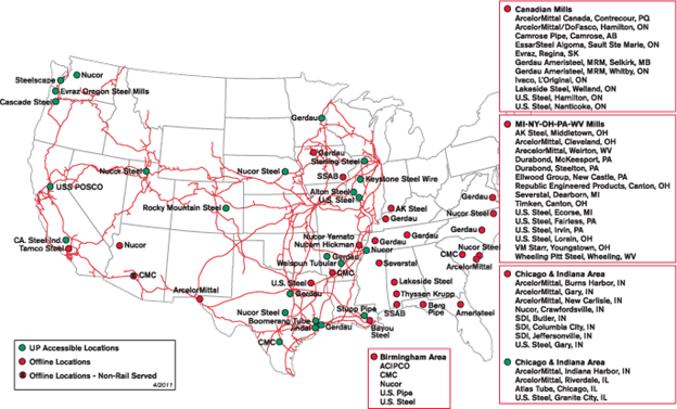
The number of steel mills has significantly declined since WWII, partly due to an increase in the amount of global competition, and partly due to the environmental and workplace regulations put in place within the US. This decline is in sharp contrast to the overall increase of steel mills in China, which has developed in recent years (Bailey et al., 2009). The current locations of steel mills in the US as of 2015 are concentrated in the eastern US. Steel mill emissions are subject to similar S emission restrictions placed on power plants (Figure 18.4).

Figure 18.3 Total S deposition (wet + dry) three-year averages through precipitation 2000-2002 compared with 2019-2021 (U.S. Environmental Protection Agency, 2023).

18.3.0.1 Table 18.2 Number of coal-burning industry units by state in the central/eastern US as of August, 2015.

State	Number of coal-burning industries
Illinois	83
Indiana	90
Iowa	28
Kansas	8
Michigan	33
Minnesota	21
Missouri	24
Nebraska	8
North Dakota	10
Ohio	119
South Dakota	2
Wisconsin	27

Figure 18.4. Steel mill locations in the USA, August, 2015 (Union Pacific, 2015)

In 1975 the total US SO₂ emissions were about 38 million tons, compared to only about 13 million tons for China. In 2000, the US had reduced their emissions to about 13 million tons, while China increased their emissions up to 35 million tons. The reduction in US S emissions helps explain the trend in sulfate deposition in the USA. In Figure 18.2; all areas of the USA experienced a reduction in sulfate deposition from 2000 to 2021. In 2000 the background levels of sulfate deposition were low enough in North Dakota that the S emission plumes of the largest coal-fired power plants located north of Bismarck and just to the north of the most northwest corner of North Dakota (Crosby, Saskatchewan) were easily seen. Currently, in general, all land in the North Central Region of the US receives only a fraction of the S from rainfall it received in 2000, which was already significantly lower than the amount deposited by rainfall in 1980.

18.4 Sulfur soil chemistry and availability

There are two main S sources in the soil; sulfate and sulfide. Through oxidation and reduction reactions mediated by microorganisms, sulfide can become sulfate. The sulfate in turn then becomes sulfide within plants and microorganisms through metabolism, and in anaerobic environments by physical chemistry Eh (redox) reactions. There are a large number of bacteria that can oxidize both sulfides and elemental S to thiosulfate and sulfate (Vidyalakshmi et al., 2009). These are categorized into two categories: chemolithotrophs, and heterotrophs. Chemolithotrophs can reproduce and metabolize only in the presence of oxidizable S compounds. Heterotrophs can selectively function as a chemolithotroph but can also conduct their normal metabolism and reproduction functions in the absence of oxidizable S. The most common chemolithotrophs are Thiobacillus sp, Thiomicrospira sp, and Thiosphaera sp. Heterotrophs include Paracoccus sp, Xanthobacter sp, Alcaligens sp, and Pseudomonas sp.

Species within the genus of chemolithotrophs vary in their ability to oxidize S and the rate of that oxidation. Some species of Thiobacillus, including T. novellus, T. acidophilus, and T. aquaesulis as well as Thiosphaera pantotroph and Thiomicrospira thyasirae are classified as heterotrophs. The implication of the large population of heterotrophic organisms abundant in soils is that oxidizable S may not be readily oxidized if there is another substrate for the microorganism to metabolize more easily and with less energy, and yet still achieve the same metabolic result. In Saskatchewan, 35 soils within the Province were assessed for presence of S oxidizing bacteria and characterized by species (Lawrence and Germida, 1991). No evidence for the presence of the obligate chemolithotrophs Thiobacillus thiooxidans or T. ferooxidans was found. The dominant populations of S oxidizing bacteria were heterotrophic and exhibited only a passive trend to oxidizing elemental S.

The general S cycling in soils is outlined in Schoenau and Germida (1992). Since S is required by plants and microorganisms, any S present in the system does not sit idly, but instead is rapidly taken up and utilized by one of these biological pools. If it is not rapidly taken up, then it can potentially be lost from the system entirely through either leaching or in a flooded system as H₂S or DMS gases. As mineral S from rainfall is added into the system, it can be utilized immediately by microorganisms, at which point it will then only become directly available to plants as it is gradually re-released through microbial mineralization as sulfate, either directly from microbial turnover or following microbial oxidation.

Plant residue decomposition can be a significant source of sulfate and, more commonly, sulfides that are oxidized by microorganisms. The amount of available S depends on how much S the plant took up, and whether it merely sufficient or excessive in S. The organic matter component of soils has an inherent C/N ratio, but it also has an intrinsic N/S ratio as well, which is usually about 10/1. As the N is mineralized, S is also released into the soil solution as an inorganic nutrient.

All of the plant available S in the soil from background S or ‘natural’ S pools, is a combination of the S received from the atmosphere originating from natural and anthropogenic sources, and the S released from inorganic S from: microorganism activity on soil organic matter, residue decomposition, any soluble sulfate salts that are present, and the slow release of S from other soil mineral sources. If the S required by the crop for growth exceeds the amount of S these background sources can supply, or the supply of these sources becomes plant-available due to excessive rainfall and subsequent leaching beyond the depth of the crop roots for uptake, supplemental S is then required.

18.5 Sulfur deficiency and the status of sulfur deficiency in the central USA

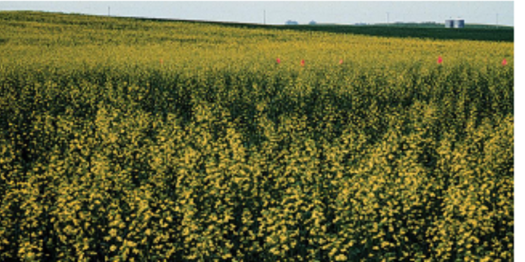
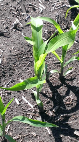
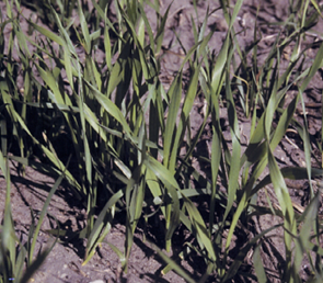
A sulfur deficiency is typically expressed in crops in the newer leaves and tissues. The most common symptom is yellowing of plant tops, but symptoms vary with the crop (Figures 18.5; 18.6; 18.7 and 18.8). Few crops are more sensitive to S than canola. Canola is a rape seed originally bred in Canada for its low erucic acid content (erucic acid is unpalatable to humans) (Gupta & Pratap, 2007). Since its early cultivation in Canada, canola has always been known for its particular sensitivity to low soil S levels and its comparatively much larger demand for S than most other crops, even other crops in the same mustard family (Figure 18.5; Grant, 1991; Franzen & Grant, 2008). The serious cultivation of canola did not begin in North Dakota until around 1994. Initially, the most severe S deficiencies were only observed on eroded hilltops and slopes, leading to the investigation of S availability across the landscape (Figure 18.6; Roberts & Bettany, 1985). Greater levels of total S were found in lower landscapes and are the result of both a higher water table, and the greater amount of S-containing organic matter present compared to upper landscape positions. A landscape-based experiment was conducted in North Dakota using different S rates and sources in 1996 (Deibert et al., 1996), and showed that although any S deficiency in canola can be catastrophic, there were large differences in the canola’s response to supplement S. The differences in responses were found to be closely tied to differences in landscape position (hilltop, slope and foot-slope positions) where the canola was being grown. Every rate of elemental S application performed better than the check, but none were nearly as effective as an application of ammonium sulfate (21-0-0-24S) at an equivalent S rate (Table 18.3).

![Figure 18.5 Early sulfur deficiency in canola.] (Pics_and_Figs/Chp_18_figs/5.png)

Figure 18.6 Sulfur deficiency in canola at flowering, from S deficient hilltop looking downslope. NDSU image.

18.5.0.1 Table 18.3 Canola yield with S rate and source, by landscape position, Rock Lake, ND. Deibert et al., 1996.

#| echo: false
#| message: false
#| warning: false
#| paged-print: false

library(gt)
library(tibble)

canola_s <- tribble(
  ~`S rate (lb/ac)`, ~`S source`, ~Buse_Hilltop, ~Barnes_Slope, ~Svea_Footslope,
   0,              "—",        30,            230,            1430,
  20,              "AS†",      1610,           1630,           1680,
  40,              "AS",       1760,           1820,           2120,
  40,              "ES",       600,            1040,           1590
)

canola <- canola_s |>
  gt() |>
  tab_header(
    title = "Table 18.3. Canola yield with S rate and source by landscape position",
    subtitle = "Rock Lake, North Dakota"
  ) |>
  tab_spanner(
    label = "Soil series / landscape position",
    columns = c(Buse_Hilltop, Barnes_Slope, Svea_Footslope)
  ) |>
  tab_spanner(
    label = "Yield (lb/acre)",
    columns = c(Buse_Hilltop, Barnes_Slope, Svea_Footslope)
  ) |>
  cols_label(
    Buse_Hilltop   = "Buse / Hilltop",
    Barnes_Slope  = "Barnes / Slope",
    Svea_Footslope = "Svea / Footslope"
  ) |>
  cols_align(
    align = "center",
    c(Buse_Hilltop, Barnes_Slope, Svea_Footslope)
  ) |>
  tab_source_note(
    source_note = "Deibert et al., 1996. †AS = ammonium sulfate; ES = elemental sulfur."
  ) |>
  opt_table_outline()

canola

Table 18.3. Canola yield with S rate and source by landscape position
Rock Lake, North Dakota
		Yield (lb/acre)
S rate (lb/ac)	S source	Soil series / landscape position
		Buse / Hilltop	Barnes / Slope	Svea / Footslope
0	—	30	230	1430
20	AS†	1610	1630	1680
40	AS	1760	1820	2120
40	ES	600	1040	1590
Deibert et al., 1996. †AS = ammonium sulfate; ES = elemental sulfur.

Figure 18.7 Sulfur deficiency in corn, NDSU image.

Figure 18.8 Sulfur deficiency in spring wheat, NDSU image.

Apart from canola, the frequency of S deficiency in other crops has steadily increased across most of the central and western regions of the United States. One reason for this steady increase is the overall increase in crop yields. In general, regardless of the crop, historically lower to modest yields required proportionally less S compared to the higher yields of the crops being produced today. A historical example of this is the historic yields of wheat grown across the prairies. Twenty years ago, spring wheat yields of 100 bushels per acre were almost unknown in North Dakota and the Canadian Prairies, whereas today they are much more commonplace. In Illinois, 250 bushels per acre corn yields were the stuff of yield contests in the 1970s; now yields exceeding that value are not, whereas today it is not uncommon to have corn yields exceeding that value. Yields of nearly all crops can increase given the environmental conditions that allow it. However, the basic principles of plant growth and nutrient demand do not change, hence: higher yields inherently require greater nutrient uptake, including and in the case of canola especially, sulfur. Sulfur deficiencies have been noted in all the states located in the North Central region, and by and large across the region the application of S is generally recommended on any coarse-textured soils with low organic matter especially soils with more than a 30 year history of corn production (Franzen and Grant, 2008; Rehm & Clapp, 2008). Spring S application as a sulfate or thiosulfate source has been the most effective in overcoming crop S deficiencies. No difference has been found between banded or broadcast applications of S, both are found to be as equally effective, as long as adequate amounts of S are applied. In a band, this usually implies that the S is applied some distance away from the seed in order to avoid salt injury; such as the 2-inch to the side and 2-inch below the seed configuration.

18.5.1 North Dakota

Since 2005, increasing cases of S deficiency on soils once thought immune to S deficiencies have been reported. As part of an N-rate study conducted from 2010 to 2014 across North Dakota, five sites were affected by S deficiency. Rescue applications of S were made at V5 and the N-rate studies were salvaged. Three of these S deficient sites consisted of silty clay loam textured soil with over five percent organic matter. Since then, it is now a standard practice in North Dakota State soil fertility experiments to apply 20 pounds per acre S as gypsum prior to planting. In 2015, several sites fertilized in this manner with S looked like ‘green islands in a sea of yellow corn’, and S deficiency symptoms affected roughly half the corn fields in eastern North Dakota (Franzen, 2015). Teboh and Zilahi-Sebess (2014) recorded a spring wheat yield increase of 7 bushels per acre along with a half point increase in grain protein from applying 20 pounds per acre S as ammonium sulfate.

18.5.2 Illinois

The frequency of S responses in Illinois has recently been increasing. In the mid to late 1970’s, Hoeft et al. (1985) conducted a series of S trials across Illinois and found that yield was increased due to and application of S at only 5 of the 82 sites observed. All the S responses were confined to soils that had low organic matter and a deep sandy profile. 25 years later, Fernandez et al. (2012), still observed S responses in several small plot and field strip corn trials on sandy soils, but this time a response to S was reported on several silt loam sites with medium organic matter levels; the mean yield increase of all the responsive sites was around 13 bushels per acre.

18.5.3 Indiana

Until recently in Indiana, all corn responses to S have been confined to coarse-textured, low organic matter soils. Sulfur response trials on wheat in 2010 also reported more widespread S deficiencies occurring, with some being reported on silt loams with moderate organic matter (Camberato & Casteel, 2010).

18.5.4 Ohio

Researchers in Ohio have also reported S responses in corn t on low organic matter, sandy soils, and as such the university recommendations now include application of S on these types of soils. As of yet in Ohio, responses have not been observed on medium or higher clay textured soils (Lentz, personal communication, August, 2015).

18.5.5 Michigan

Sulfur deficiency has also not been a historic problem in Michigan. This is probably because of the large amounts of atmospheric S deposition from the Great Lakes coal/oil/gas fired industries (until their recent reduction) (Vitosh et al., 1994). The exception to this was some documented S deficiencies on low organic matter, sandy soils in kidney bean and corn were noted.

18.5.6 Wisconsin

In Wisconsin, S deficiency in alfalfa on sandy, low organic soils has been reported and researched for over thirty years (Hoeft et al., 1973), and continues to be a problem for alfalfa producers in the southwest region of Wisconsin (Laboski personal communication, August, 2015). Sulfur deficiency can also be observed in corn grown on sandy and loamy soils and also on the shallow silt loam soils of both central and western Wisconsin (< 30 inches of soil over bedrock).

18.5.7 Iowa

In Iowa S deficiencies were reported for the first time in 2005, when alfalfa yields were dramatically increased with additional S fertilization (Sawyer et al., 2009). This result was followed in 2006 on corn grown on similar sites also suspected of having a S deficiency, where the application of 40 pounds per acre S as calcium sulfate applied during early corn growth increased yields by 38 bu/acre on average in five out of the six sites (Sawyer et al., 2009). These successful studies were expanded in 2007 and 2008, across the sites representing the major soils across the north-central Iowa region. Sulfur increased corn yields at 17 of 20 sites in 2007 and 11 of 25 sites in 2008. Average corn yield increases were about 15 bushels per acre on fine-textured sites and 28 bushels per acre on coarse-textured soil sites. Overall, between 2006 and 2013, 47 percent of the 110 S rate trials conducted in Iowa showed a corn yield response to S application (Rueber & Sawyer, 2013).

18.5.8 Missouri

In Missouri S deficiency has only been observed on low organic matter, sandy soils (P. Scharf, personal communication, August, 2015). No increase or expansion of S deficiency in corn has been noted.

18.5.9 Kansas

Kansas has had a long history of S deficiency on low organic matter, sandy soils (D. Mengel, personal communication, August, 2015). Yield increases to S in wheat, grain sorghum, alfalfa, bromegrass and tall fescue have all been recorded. Most of these studies were conducted on low organic matter soils, except bromegrass which responded to S on soils with organic matter greater than 3 percent (Lamond, 1997). Until recently, yield increases due to S application were confined to traditionally S-deficient soils. However, in 2012, yield increases to S application were recorded in soils with greater clay content (Widmar & Ruiz Diaz, 2012).

18.5.10 Minnesota

In Minnesota, for many years an application of S has been recommended for sandy, low organic matter soils (Rehm & Clapp, 2008). With a series of studies beginning in 1999, corn yield responses to S were recorded in loam and silt loam soils, but not on silty clay loam textured soil (Rehm, 2005). Kim et al. (2013) expanded on previous work and found additional corn yield response to S on higher organic matter loam soils. Although it is unusual to experience a soybean yield increase to S, Kaiser and Kim (2013) increased soybean yield only on low organic matter (<2%) silt loam soil.

18.5.11 Nebraska

In Nebraska, the irrigation water typically has enough sulfate-S to cover most of the crops needs. Despite this, applying S through the irrigation pivot is still a common practice in many areas of Nebraska, including on both the sand hills region (the irrigated sands of the north central region of Nebraska), and on the sandy soils of the river valleys in the central and southern fields of Nebraska (Ferguson, Wortman & Shapiro, personal communications, August, 2015). As much as 50 lb/acre of S is applied annually through the irrigation pivot in some fields, as either ammonium thiosulfate, ammonium sulfate, or sulfur-magnesium through the irrigation pivot is applied annually to some fields.

18.6 Diagnostic value of S soil tests

Tabatabai (1996) reviewed a large number of methods for S determination in soils. He noted that, based on relationships found by Probert (1976) between, sulfate extracted by Ca(H₂PO₄)₂, and plant uptake, it is generally accepted that the monocalcium phosphate extraction method is the most correlated method of S determination to crop production. As a result, this test is the most commonly used analysis by soil laboratories across the North Central USA region, and can be used to guide growers on their soil S status. Research by others in the 1960’s and the early 1970’s however, only partly supported the utility and accuracy of using monocalcium phosphate as an extractant (Fox et al., 1964; Hoeft et al., 1973). Hoeft et al. (1973) found that the monocalcium phosphate with 2N acetic acid performed the best out of all the extractants examined. Contrastingly they also found that the monocalcium phosphate without 2N acetic acid was very poor at predicting alfalfa yield based on the extracted soil sulfate-S. Soon after this report was published, however, practitioners found that using the acetic acid version of the extractant was impractical to use compared to the water-based monocalcium phosphate extractant. Because of this, with rare exception, presently most soil laboratories do not use the acetic acid based extractant. Despite the overwhelming adoption of the monocalcium phosphate extractant by laboratories, overall, it does not correlate to the yield responses of most crops to sulfate-S, and therefore is considered to be “non-diagnostic”. All other extractants tested to date have similarly been non-diagnostic across the variety of soils in which they have been tested.

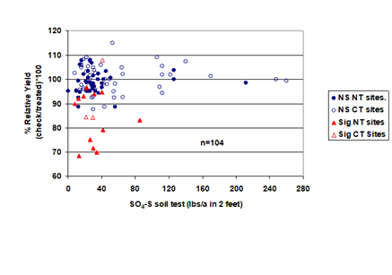
In Iowa from 2007 to 2009, experiments on the effects of an S application to corn showed that the quantity of soil extractable sulfate-S was not correlated to the yield response in the check plots. For example, extractable sulfate concentrations higher than 10 ppm should have denoted soil where you would not see a response to S, however, many of these sites responded to S. The non-relationship of the current sulfate-S soil test with corn yield is shown in Figure 18.9 (Sawyer et al., 2009).

Figure 18.9 Relative corn yield in relation to sulfate-S soil test, Iowa (Sawyer et al., 2009).

At both Brookings and Beresford, SD, extractable sulfate-S values were also non-diagnostic based on 10 years of data compiled from various sulfur fertilization trials (Gelderman, unpublished data). Despite the soil always testing low for S over the 10-year period, there was no documented response to S. At Beresford, only a 4 bu/acre average response was documented. A visual depiction of the relationship between the sulfate-S soil test levels and the corn yield responses in SD over 17 years is shown in Figure 18.10. The correlation between the extractable sulfate-S values and canola yield responses in North Dakota has also been consistently so low (Lukach, personal communication, 2012). In 2014 in North Dakota, S fertilization resulted in spring wheat yield increases even on soil with a ‘high’ beginning soil sulfate-S test value (Teboh and Zilhi-Sebess, 2014).

Figure 18.10 Relative corn yield in relation to sulfate-S soil test, South Dakota, 1990-2007 (Gelderman, unpublished data).

In 1991 a S-sulfate soil test was developed using KCl as an extractant by Blair et al. (1991) which showed a positive relationship between extracted sulfate-S and crop yield response. On closer examination of the data however, the prediction formula is based on two different sets of soils: soils that have variable yields and yet nearly always have a low S soil test, and soils that are high yielding over a wide range of extractable S values. The combined results of the two data sets together can be statistically manipulated to form a steep quadratic curve, with a nearly vertical component from one soil group, and an unresponsive horizontal component from the other soil group. Kim and colleagues (2013) showed no relationship between KCL extracted sulfate-S test results and yield in Minnesota.

One reason why a better sulfur soil test has not been developed in the US is that before 2005, S deficiencies were not widespread. Instead, they were localized in smaller geographic areas, and were considered to be of only a minor importance. Currently, the increasingly large number of S deficiencies across the North Central Region has provided a stage for further testing and the development of new ideas for testing soil for S deficiency and predicting crop response to added S, that historically could not have been developed.

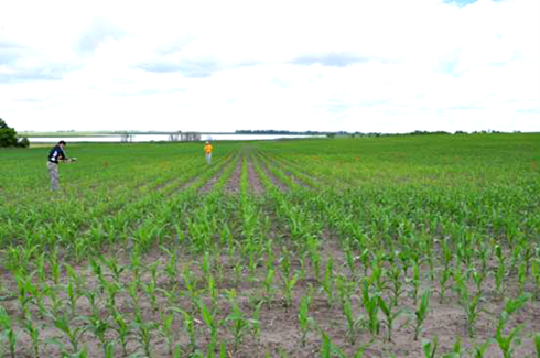
One new method of predicting corn yield response to added S is the use of active-optical sensors. Active optical sensors have been used to determine the need for a side-dress application of N in corn. The rate is determined by establishing a non-limiting N area within the field of interest. Several nitrogen rate studies in North Dakota have indicated the potential use of such an N non-limiting area to also reveal potential S deficiency (Figure 18.11). For example, if N in a crop is very deficient, there are signals within the crop that will result in the deconstruction of N containing compounds, such as proteins, and the relocate these compounds to areas of newer growth. If both N and S are deficient, the S is also relocated along with the N in these compounds, since S is naturally present in several amino acids and other N containing compounds. If N is not deficient, and S is deficient, there is no such signal in the crops to deconstruct these compounds and relocate them. The result is that when N is adequately supplied, S deficiency symptoms are then intensified. For example, in a non-limiting N area within a S deficient field, the non-limiting N area will be the most yellow area of the field. If this is detected either visually or with an active-optical sensor, S should then be applied immediately to remedy the condition (Sharma et al., 2015).

Figure 18.11 Sulfur-deficient N rate study near Oakes, ND, spring 2014. Yellowest plots are high N rates. Greenest plots are low N rates. Following S application, the high N rate plots became the greenest and check plots were least green. The grower cooperator had applied 10 pound per acre S in a 2X2 band as ammonium thiosulfate to corn surrounding our experimental area (foreground; Sharma et al., 2015).

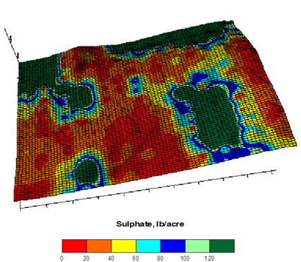
If in the future a more suitable S soil test is found, the inherent variability of S within a given field will still be a concern. In North Dakota, extractable sulfate-S values are one of the most variable nutrients that are analyzed in site-specific nutrient management experiments. Sulfur values in soil cores collected down to 2 feet in depth can vary from under 10 pounds S per acre to nearly 1000 pounds S per acre within a 40-acre field (Figure 18.12). Therefore, regardless of what method is used to try and predict the S status of soils in the future, sampling for S while still considering its mobility in the soil will most likely still be strongly advised.

Figure 18.12. Variability of sulfate-S analyzed from a 110-foot grid over a 40-acre field near Valley City, ND. High sulfate areas tend to be local depressions and lowest sulfate are in low organic matter upland soils, usually, but not always associated with coarser textured soils.

18.7 Alternative S prediction strategies

Across all the states with substantial regions that have a history of repeated seasons of S deficiency in some soils, extractable soil S is usually a factor within the fertility recommendation equation. Kansas has such an equation (Lamond, 1997), as does Nebraska (although Nebraska’s recommendations are in the form of a chart, but instead listing both the soil test sulfate value and the organic matter as factors) (Shapiro et al., 2008). In North Dakota however, growers are urged to track both fall and spring rainfall, along with the winter snowmelt. If the amount of precipitation during this period is greater than normal, then S deficiencies on both small grains and corn should be anticipated; and a spring application of S should be made to prevent a potential deficiency, regardless of the soil test value. In-season plant tissue analysis for S paired and collected from an area of the field where S is suspected to be deficient and an area where the plants appear to be healthy can be a helpful diagnostic tool. An unpaired plant tissue sample from a field is typically discouraged because of: varietal variation, the potential spatial variability of individual plant S status, and the wide variation in S concentration from different critical level nutrient charts (Mallarino, 2013).

18.8 Sulfur amendment sources and application

Manure can be an abundant and readily available S amendment for some producers. The typical S content of dry manure can vary from 1 to 3 pounds of S per ton, while the S in liquid manure typically varies anywhere from 4 to 9 pounds of S per 1,000 gallons. Manure is an organic source (not to be confused with the “organic” terminology you might see on a food label at the grocery store, but organic in terms of its carbon chemistry) of S. As such, some fraction of the total S may be in an immediately plant-available form, while the majority may still need to undergo further decomposition for the S to become plant available. The fraction of the total S in manure that is considered to be plant available can vary from <1 to 2 pounds of S per ton for dry manure sources, and 2 to 5 pounds of S per 1,000 gallons for liquid manure sources (Lamond, 1997). A manure analysis is required in order to best estimate the total S content of the manure. Referencing the most recent state manure nutrient availability report published by your state is also highly recommended. The S content of the most common S fertilizers used across the region are listed in Table 18.4. All of the materials in Table 18.4 have been found to be highly effective in increasing crop yields when S is deficient, applied either preplant or in-season, by researchers in the northern Great Plains.

Elemental S is not listed as a standalone fertilizer, because researchers who have included it in their studies have found that although crop yields can be increased with its use, other products are proven to be far more effective. A full discussion of the problems of oxidation of elemental S to sulfate is provided in Franzen and Grant (2008). The most common management practice to ensure the efficacy of S fertilizers is spring application. Across the region the period of highest soil moisture as well as the greatest potential for fertility losses via leaching is in the early spring prior to planting. As such, the worst possible time to apply either sulfate or thiosulfate fertilizers is in the fall. This does however, put enormous pressure on fertilizer suppliers managing the logistics of only applying S fertilizers in the spring.

Ammonium sulfate, potassium magnesium sulfate, the Mosaic MES products, gypsum and potassium sulfate are all dry granular products. One of the problems of applying ammonium sulfate twenty years ago was the segregation of the fertilizer granules when smaller crystal/granule sizes were used. Ammonium sulfate granules that are similar in size to KCl, phosphate fertilizers and urea are now provided by most manufacturers to minimize segregation during blending and to allow for a more even application. Gypsum formulations that can easily be blended with other dry fertilizers are currently under development, but there are some manufacturers that have been able to formulate a granule that is compatible with other fertilizer blending products. Ammonium thiosulfate and potassium thiosulfate are both liquid fertilizers, with ammonium thiosulfate currently being sold more. Much of the ammonium thiosulfate fertilizer is applied through an irrigation pivot. However, sizable tonnage is also applied as a 2X2 band at planting and mixed with UAN solutions for a dribbled or coulter applied side-dress application. Ammonium thiosulfate has been shown to cause some reduction to stands in some studies when it is applied directly with the seed at low rates, with much larger reductions occurring at higher rates (Rehm, 2005).

18.8.0.1 Table 18.4 Major effective fertilizer S sources used in the US Great Plains, 2015.

Fertilizer	% N	% P₂O₅	% K₂O	% S
Ammonium sulfate	20–21	0	0	24
Ammonium thiosulfate	12	0	0	26
Calcium sulfate/hydrated (Gypsum)	0	0	0	18.6
Potassium sulfate	0	0	50	17.6
Potassium thiosulfate	0	0	20	17
Potassium magnesium sulfate	0	0	22	22
MES 15 (50% ammonium sulfate, 50% elemental S)	13	33	0	15

Unless rainfall totals for the fall, winter and early spring months are low, S applications should still be spring applied. In a recent Illinois study, only 6% of the fall applied S-sulfate was present in 0–36-inch soil profile, compared to 40% remaining when it was spring applied (Degryse et al., 2015).

18.9 Sulfur references

• Andreae, M. O. (1990). Ocean-atmosphere interactions in the global biogeochemical sulfur cycle. Marine Chemistry, 30(1-3), 1-29. https://doi.org/10.1016/0304-4203(90)90059-L

• Arndt, J. L., & Richardson, J. L. (1989). Geochemistry of hydric soil salinity in a recharge-throughflow-discharge prairie-pothole wetland system. Soil Science Society of America Journal, 53(3), 848-855. https://doi.org/10.2136/sssaj1989.03615995005300030030x

• Bailey, B., Huff, P., Tianjie, J., Matthews, P., Rothschild, R., Swerdlow, J., Wang, Y., & Wegman, R. (2009). An assessment of environmental regulation of the steel industry in China. Alliance for American Manufacturing. https://www.americanmanufacturing.org/research/

• Barnes, I., Hjorth, J., & Mihalopoulos, N. (2006). Dimethyl sulfide and dimethyl sulfoxide and their oxidation in the atmosphere. Chemical Reviews, 106(3), 940-975. https://doi.org/10.1021/cr020529+

• Blair, G. J., Chinoim, N., Lefroy, R. D. B., Anderson, G. C., & Crocker, G. J. (1991). A soil sulfur test for pastures and crops. Australian Journal of Soil Research, 29(5), 619-626. https://doi.org/10.1071/SR9910619

• Bluth, G. J. S., Dorian, S. D., Schnetzler, C. C., Krueger, A. J., & Walter, L. S. (1992). Global tracking of the SO₂ clouds from the June 1991 Mount Pinatubo eruptions. Geophysical Research Letters, 19(2), 151-154. https://doi.org/10.1029/91GL02792

• Camberato, J., & Casteel, S. (2010, April 13). Keep an eye open for sulfur deficiency in wheat. Purdue University Department of Agronomy Soil Fertility Update. https://ag.purdue.edu/agry/extension/Documents/indiana-sulfur-deficiency-wheat.pdf

• Degryse, F., da Silva, R. C., Baird, R., & McLaughlin, M. (2015, November). Sulfur uptake by corn from fall- or spring-applied S-34 labelled fertilizer. Soil Science Society of America Abstracts, Paper 95123. https://scisoc.confex.com/scisoc/2015am/webprogram/Paper95123.html

• Deibert, E. J., Halley, S., Utter, R. A., & Lukach, J. (1996). Canola response to sulfur fertilizer applications under different tillage and landscape positions. 1996 Annual Report to USDA/CSREES/Special Programs North Central Region Canola and North Dakota Oilseed Council.

• Eriksson, E. (1952). Composition of atmospheric precipitation. II. Sulfur, chloride, iodine compounds. Tellus, 4(3), 280-303. https://doi.org/10.3402/tellusa.v4i3.8535

• Fernandez, F. G., Ebelhar, S., Greer, K., & Brown, H. (2012). Corn response to sulfur in Illinois (FREC Report No. 358). Illinois Fertilizer and Chemical Association. https://www.ifca.com/media/files/frec_358_fernandez_2012_report.pdf

• Fernihough, A., & O’Rourke, K. H. (2014). Coal and the European industrial revolution (University of Oxford Discussion Papers in Economic and Social History, Vol. 124). University of Oxford. http://www.economics.ox.ac.uk/materials/papers/13183/Coal%20-%20O’Rourke%20124.pdf

• Fox, R. L., Olson, R. A., & Rhoades, H. F. (1964). Evaluating the sulfur status of soils by plant and soil tests. Soil Science Society of America Proceedings, 28, 243-246. https://doi.org/10.2136/sssaj1964.03615995002800020037x

• Franzen, D. W. (2003). Managing saline soils in North Dakota (Extension Circular SF-1087). North Dakota State University Extension.

• Franzen, D. W. (2015, June 18). Sulfur deficiency in corn pandemic. Crop and Pest Report, 7. North Dakota State University Extension.

• Franzen, D. W., & Grant, C. A. (2008). Sulfur response based on crop, source and landscape position. In J. Jez (Ed.), Sulfur: A missing link between soils, crops, and nutrition (pp. 105-112). Agronomy Monograph No. 50. ASA-CSSA-SSSA.

• Giblin, A. E., & Wieder, R. K. (1992). Sulphur cycling in marine and freshwater wetlands. In R. W. Howarth, J. W. B. Stewart, & M. V. Ivanov (Eds.), Sulphur cycling on the continents, wetlands, terrestrial ecosystems, and associated water bodies (SCOPE 48). Scientific Committee on Problems of the Environment (SCOPE). http://www.scopenvironment.org/downloadpubs/scope48/

• Graf, H.-F., Feichter, J., & Langmann, B. (1997). Volcanic sulfur emissions: Estimates of source strength and its contribution to the global sulfate distribution. Journal of Geophysical Research: Atmospheres, 102(D9), 10727-10738. https://doi.org/10.1029/96JD03265

• Grant, C. A. (1991). Sulphur requirements of canola. Sulphur in Agriculture, 15, 3-6.

• Gupta, S. K., & Pratap, A. (2007). Canola: History, origin and evolution. In J. Janick (Ed.), Advances in Botanical Research (Vol. 45, pp. 1-20). Elsevier. https://doi.org/10.1016/S0065-2296(07)45001-2

• Halmer, M. M., Schmincke, H.-U., & Graf, H.-F. (2002). The annual volcanic gas input into the atmosphere, in particular into the stratosphere: A global data set for the past 100 years. Journal of Volcanology and Geothermal Research, 115(3-4), 511-528. https://doi.org/10.1016/S0377-0273(01)00318-3

• Hoefgen, R., & Hesse, H. (2008). Sulfur and cysteine metabolism. In J. Jez (Ed.), Sulfur: A missing link between soils, crops, and nutrition (Agronomy Monograph No. 50, pp. 83-104). ASA, CSSA, and SSSA. Madison, WI. https://doi.org/10.2134/agronmonogr50.c6

• Hoeft, R. G., Walsh, L. M., & Keeney, D. R. (1973). Evaluation of various extractants for available soil sulfur. Soil Science Society of America Journal, 37(3), 401-404. https://doi.org/10.2136/sssaj1973.03615995003700030032x

• Hoeft, R. G., Sawyer, J. E., Vanden-Heuvel, R. M., Schmitt, M. A., & Brinkman, G. S. (1985). Corn response to sulfur on Illinois soils. Journal of Fertilizer Issues, 2, 95-104.

• Kaiser, D. E., & Kim, K.-I. (2013). Soybean response to sulfur fertilizer applied as a broadcast or starter using replicated strip trials. Agronomy Journal, 105(4), 1189-1198. https://doi.org/10.2134/agronj2012.0459

• Kennedy, K. A. (1994). Early-Holocene geochemical evolution of saline Medicine Lake, South Dakota. Journal of Paleolimnology, 10(1), 69-84. https://doi.org/10.1007/BF00682507

• Kim, K.-I., Kaiser, D. E., & Lamb, J. (2013). Corn response to starter fertilizer and broadcast sulfur evaluated using strip trials. Agronomy Journal, 105(2), 401-411. https://doi.org/10.2134/agronj2012.0350

• Joeckel, R. M., & Ang Clement, B. J. (2005). Soils, surficial geology, and geomicrobiology of saline-sodic wetlands, North Platte River Valley, Nebraska, USA. Catena, 61(1), 63-101. https://doi.org/10.1016/j.catena.2005.02.009

• Joshi, M. M., & Jones, G. S. (2009). The climatic effects of the direct injection of water vapour into the stratosphere by large volcanic eruptions. Atmospheric Chemistry and Physics, 9(17), 6109-6118. https://doi.org/10.5194/acp-9-6109-2009

• Lamond, R. (1997, reissued 2014). Sulphur in Kansas (Kansas State University Circular MF-2264). Kansas State University Research and Extension. https://www.bookstore.ksre.ksu.edu/pubs/MF2264.pdf

• Mallarino, A. P. (2013). Interpretation of plant tissue test results for phosphorus and potassium in corn and soybean. In NCERA-13 2013 Workshop Proceedings. http://www.agronext.iastate.edu/soilfertility/info/Mallarino_Tissue%20PK%20testing_NCERA-13%20Wkshop%202013.pdf

• Manahan, S. E. (2013). Environmental and toxicological chemistry (4th ed.). CRC Press, Taylor & Francis Group.

• Mokyr, J. (1998). The Second Industrial Revolution 1870-1914. Northwestern University. http://faculty.wcas.northwestern.edu/~jmokyr/castronovo.pdf

• Murray, R. C. (1964). Origin and diagenesis of gypsum and anhydrite. Journal of Sedimentary Petrology, 34(3), 512-523.

• NASA Earth Observatory. (2010, March 13). Hydrogen sulfide emissions along the Namibian coast [Satellite image]. NASA. https://earthobservatory.nasa.gov/images/43143/hydrogen-sulfide-emissions-along-the-namibian-coast

• Parat, F., Holtz, F., & Streck, M. J. (2011). Sulfur-bearing magmatic accessory minerals. Reviews in Mineralogy & Geochemistry, 73, 285-314. https://doi.org/10.2138/rmg.2011.73.11

• Probert, M. E. (1976). Studies on ‘available’ and isotopically exchangeable sulphur in some north Queensland soils. Plant and Soil, 45(2), 461-475. https://doi.org/10.1007/BF00010933

• Rehm, G. W. (2005). Sulfur management for corn growth with conservation tillage. Soil Science Society of America Journal, 69(3), 709-717. https://doi.org/10.2136/sssaj2005.0709

• Rehm, G. W., & Clapp, J. G. (2008). Sulfur in a fertilizer program for corn. In J. Jez (Ed.), Sulfur: A missing link between soils, crops, and nutrition (pp. 143-153). Agronomy Monograph No. 50. ASA-CSSA-SSSA.

• Rickard, D. (2012). Sulfidic sediments and sedimentary rocks. A. J. van Loon (Ed.). Elsevier.

• Roberts, T. L., & Bettany, J. R. (1985). The influence of topography on the nature and distribution of soil sulfur across a narrow environmental gradient. Canadian Journal of Soil Science, 65(3), 419-434. https://doi.org/10.4141/cjss85-042

• Rueber, D., & Sawyer, J. E. (2013). Corn and soybean response to sulfur application rate (Iowa State Research Farm Progress Report RFR‑A12103). Iowa State University Digital Press. https://iastatedigitalpress.com/farmreports/article/951/galley/824/view/

• Sawyer, J. E., Lang, B., Barker, D. W., & Cummins, G. (2009, November). Dealing with sulfur deficiencies in crop production: The Iowa experience [Conference paper]. In North Central Extension‑Industry Soil Fertility Conference Proceedings (Vol. 25, pp. 64-71). Iowa State University.

• Schoenau, J. J., & Germida, J. J. (1992). Sulphur cycling in upland agricultural systems. In Sulphur cycling on the continents: Wetlands, terrestrial ecosystems and associated water bodies (pp. 261-277). In R. W. Howarth, J. M. Cotman, J. G. Titus, & B. J. Presser (Eds.), SCOPE No. 48. John Wiley & Sons.

• Shapiro, C. A., Ferguson, R. B., Hergert, G. W., Wortmann, C. S., & Walters, D. T. (2008). Fertilizer suggestions for corn (University of Nebraska Extension Circular EC117). University of Nebraska-Lincoln Extension. http://ianrpubs.unl.edu/live/ec117/build/ec117.pdf

• Sharma, L. K., Bu, H., Denton, A., & Franzen, D. W. (2015). Active-optical sensors using red NDVI compared to red edge NDVI for prediction of corn grain yield in North Dakota, U.S.A. Sensors, 15(11), 27,832-27,853. https://doi.org/10.3390/s151127832

• Skarie, R. L., Richardson, J. L., McCarthy, G. J., & Maianu, A. (1987). Evaporite mineralogy and groundwater chemistry associated with saline soils in eastern North Dakota. Soil Science Society of America Journal, 51(5), 1372-1377. https://doi.org/10.2136/sssaj1987.03615995005100050048x

• Tabatabai, M. A. (1996). Sulfur. In J. M. Bartels (Ed.), Methods of soil analysis. Part 3: Chemical methods (pp. 921-960). Soil Science Society of America, American Society of Agronomy.

• Teboh, J. M., & Zilahi-Sebess, S. (2014). Sulfur application increased wheat grain yield in a fertilizer rate study at Carrington. In Carrington Research Extension Center: A report of agricultural research and extension in central North Dakota (Vol. 55, pp. 19-20). NDSU Agricultural Experiment Station.

• Textor, C., Graf, H. F., Timmreck, C., & Robock, A. (2003). Emissions from volcanoes. In C. Granier, C. Reeves, & P. Artaxo (Eds.), Emissions of chemical compounds and aerosols in the atmosphere (pp. 32). Kluwer Academic Publishers.

• Theophrastus. (300 BC/1956). On stones (E. R. Caley & J. C. Richards, Trans.). The Ohio State University Press. https://ohiostatepress.org/index.htm?books/book%20pages/Caley%20Theophrastus.html

• Union Pacific. (2015, August). Steel mill locations in the USA. http://www.up.com/customers/ind-prod/metals/steel-mill/index.htm (Page no longer available; accessed August 2015)

• U.S. Environmental Protection Agency. (2015). Acid Rain Program. https://www.epa.gov/airmarkets/programs/arp/

• U.S. Environmental Protection Agency. (2023, January). Sulfur deposition map [Web figure]. In Acid deposition figures. Power Sector Programs Progress Reports. U.S. Environmental Protection Agency. https://www3.epa.gov/airmarkets/progress/reports/acid_deposition_figures.html

• Vidyalakshmi, R., Paranthaman, R., & Bhakyaraj, R. (2009). Sulphur oxidizing bacteria and pulse nutrition - A review. World Journal of Agricultural Sciences, 5(2), 270-278.

• Vitosh, M. L., Warncke, D. D., & Lucas, R. E. (1994). Secondary and micronutrients for vegetables and field crops (Michigan State University Extension Circular E-486, Rev. Aug. 1994). Michigan State University.

• Weeks, S. J., Currie, B., Bakun, A., & Peard, K. R. (2004). Hydrogen sulphide eruptions in the Atlantic Ocean off southern Africa: Implications of a new view based on SeaWiFS satellite imagery. Deep-Sea Research Part I: Oceanographic Research Papers, 51(2), 153-172. https://doi.org/10.1016/j.dsr.2003.10.004

• Whittemore, D. O. (2000). Water quality of the Arkansas River in southwest Kansas. Kansas Geological Survey. Report to the Kansas Water Office (Contract No. 00-113), Upper Arkansas River Corridor Study.

• Widmar, A., & Ruiz Diaz, D. A. (2012). Evaluation of macro- and micronutrients for double-crop soybean after wheat. In Kansas Fertilizer Research 2012 (pp. 3-6). Kansas State University. http://www.k-state.edu/historicpublications/Pubs/SRP1085.pdf

• Yinke, D. (2011). Ancient Chinese inventions (English translation). Cambridge University Press.